Beat phenomenon

import vibration_toolbox as vtb

import matplotlib.pyplot as plt
from ipywidgets import interact, interactive, widgets
from IPython.display import Audio, display

# %matplotlib inline

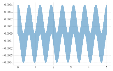
In this notebook we will investigate a phenomena that occurs when the driving frequency becomes close to the system’s natural frequency.

For zero initial conditions, the response is given by the equation:

\begin{equation} x(t) = \frac{2f_0}{\omega^2_n - \omega^2} sin\Big(\frac{\omega_n - \omega}{2} t\Big) sin\Big(\frac{\omega_n + \omega}{2}t\Big) \end{equation}

Since \((\omega_n - \omega)\) is small, \((\omega_n + \omega)\) is large in comparison and \(sin[(\omega_n - \omega)/2]t\) oscillates with a longer period than \(sin[(\omega_n + \omega)/2]t\). The result is a rapid oscillation with slowly varying amplitude that is called a beat.

The system defined in the function bellow has a a natural frequency \(\omega_n = 1000 \ rad/s\).

You can change the excitation frequency moving the slide ‘wdr’ and hear the resulting sound.

When you get close to the natural frequency you will be able to recognize the beats.

@interact(wdr=widgets.FloatSlider(min=900.1, max=1100.1, step=1, value=1100))
def f(wdr):
    t, a = vtb.forced_analytical(m=1, k=10**6, x0=0, v0=0, wdr=wdr, F0=200, tf=5)
    display(Audio(data=a, rate=1/0.000125))
    plt.plot(t, a, alpha=0.5)
    plt.show()

w = interactive(f,wdr = (900.1,1100.1,1));
display(w);

f(wdr=10)

w = f(wdr=10)

@interact
def f2(wdr=10):
    t, a = vtb.forced_analytical(m=1, k=10**6, x0=0, v0=0, wdr=wdr, F0=200, tf=5)
    # display(Audio(data=a, rate=1/0.000125))
    plt.plot(t, a, alpha=0.5)
    plt.show()
    return

w = f2(wdr=10.0)
interact(w,wdr=10.)

<ipywidgets.widgets.interaction._InteractFactory at 0x111e66f28>

interactive(f2,wdr=10.0)