Single Degree of Freedom Systems (vibration_toolbox.sdof)

The vibration_toolbox.sdof

sdof – Single Degree of Freedom Functions

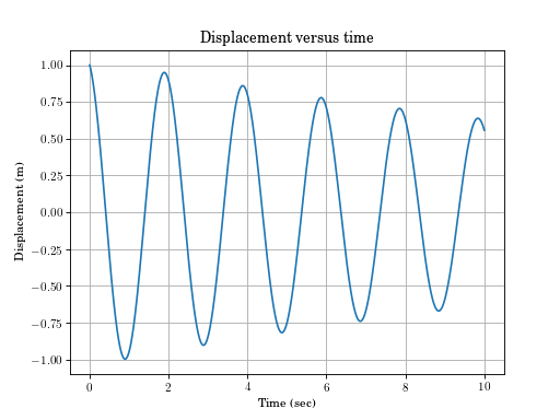
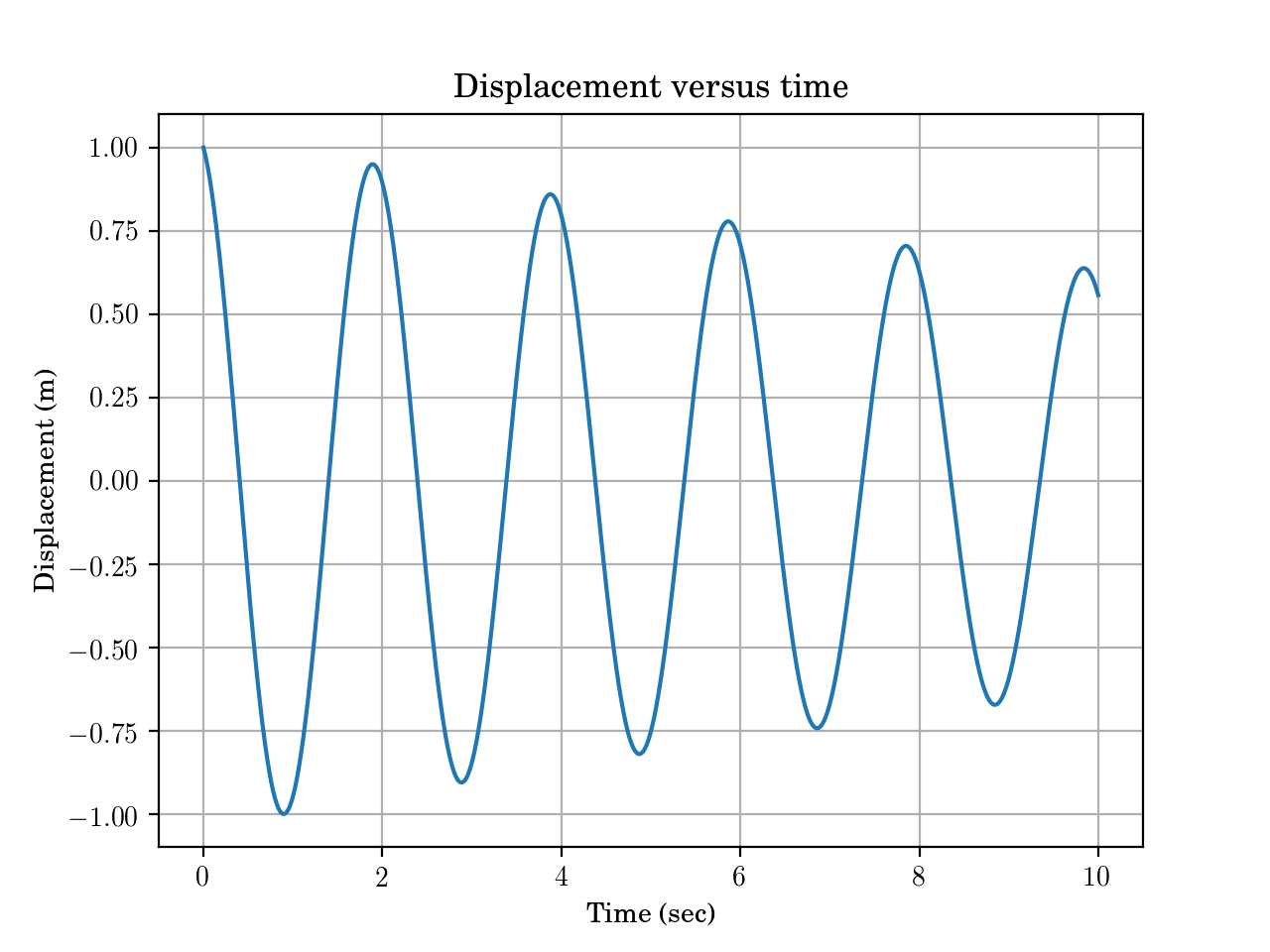
sdof.free_response(m=10, c=1, k=100, x0=1, v0=-1, max_time=10)

Free response of a second order linear oscillator.

Returns t, x, v, zeta, omega, omega_d and A resulting from the free response of a second order linear ordinary differential equation defined by \(m\ddot{x} + c \dot{x} + k x = 0\) given initial conditions \(x_0\) and \(\dot{x}_0 = v_0\) for \(0 < t < t_{max}\)

Parameters

m, c, kfloats, optional

mass, damping coefficient, stiffness

x0, v0: floats, optional

initial displacement, initial velocity

max_time: float, optional

end time for \(x(t)\)

Returns

t, x, vndarrays

time, displacement, and velocity

zeta, omega, omega_d, Afloats

damping ratio, undamped natural frequency, damped natural frequency, Amplitude

Examples

(Source code, png, hires.png, pdf)

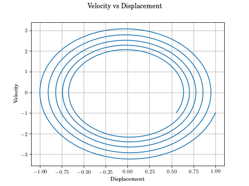
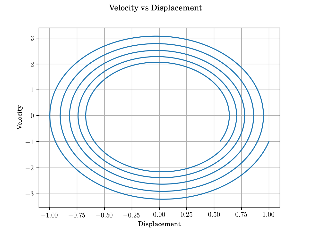
sdof.phase_plot(m=10, c=1, k=100, x0=1, v0=-1, max_time=10)

Phase plot of free response of single degree of freedom system.

For information on variables see free_response.

Parameters

m, c, k: floats, optional

mass, damping coefficient, stiffness

x0, v0: floats, optional

initial displacement, initial velocity

max_time: float, optional

end time for \(x(t)\)

Examples

(Source code, png, hires.png, pdf)

sdof.phase_plot_i(max_time=(1.0, 200.0), v0=(-100, 100, 1.0), m=(1.0, 100.0, 1.0), c=(0.0, 1.0, 0.1), x0=(-100, 100, 1), k=(1.0, 100.0, 1.0))

Interactive phase plot of free response of SDOF system.

phase_plot_i is only functional in a Jupyter notebook.

Parameters

m, c, k: floats, optional

mass, damping coefficient, stiffness

x0, v0: floats, optional

initial displacement, initial velocity

max_time: float, optional

end time for \(x(t)\)

sdof.time_plot_i(max_time=(1.0, 100.0), x0=(-100, 100), v0=(-100, 100), m=(1.0, 100.0), c=(0.0, 1.0, 0.02), k=(1.0, 100.0))

Interactive single degree of freedom free reponse plot in iPython.

time_plot_i is only functional in a Jupyter notebook.

Parameters

m, c, k: floats, optional

mass, damping coefficient, stiffness

x0, v0: floats, optional

initial displacement, initial velocity

max_time: float, optional

end time for \(x(t)\)

sdof.forced_response(m=10, c=0, k=100, x0=1, v0=0, wdr=0.5, F0=10, max_time=100)

Harmonic response of SDOF system.

Returns the the response of an underdamped single degree of freedom system to a sinusoidal input with amplitude F0 and frequency \(\omega_{dr}\).

Parameters

m, c, k: float, optional

Mass Damping, and stiffness

x0, v0: float, optional

Initial conditions

wdr: float, optional

Force frequency

F0: float, optional

Force magnitude

max_time: float, optional

End time

Returns

t, x, v: array

Time, displacement and velocity

Examples

>>> import vibration_toolbox as vtb
>>> t, x, v = vtb.forced_response(m=10, c=0, k=100, x0=1, v0=0, wdr=0.5, F0=10, max_time=100)
>>> plt.plot(t,x,t,v)
[<matplotlib.lines.Line2D ...

sdof.transmissibility(zs=array([ 0.05, 0.1, 0.25, 0.5, -0.75]), rmin=0.0, rmax=2.0)

Plot transmissibility ratio for SDOF system.

Parameters

zs: array

Array with the damping values

rmin, rmax: floats

Minimum and maximum frequency ratios

Returns

r: float array

Array containing the values for the frequency ratio

D: float array

Array containing the values for displacement

F: float array

Array containing the values for force

Plot with Displacement transmissibility ratio and force transmissibility ratio

Examples

>>> import vibration_toolbox as vtb
>>> r, D, F = vtb.transmissibility(zs=[0.1, 0.2], rmin=0, rmax=2)

sdof.rotating_unbalance(m, m0, e, zs, rmin, rmax, normalized=True)

Plot displacement of system responding to rotating unbalance.

Parameters

m: float

Mass of the system

m0, e: float

Mass and eccentricity of the unbalance.

zs: array

Array with the damping values

rmin, rmax: float

Minimum and maximum frequency ratio

normalized: bool

If true, the displacement is normalized (m*X/(m0*e))

Returns

r: Array

Array containing the values for the frequency ratio

Xn: Array

Array containing the values for displacement

Plot with Displacement displacement and phase for a system with rotating unbalance.

Examples

>>> import vibration_toolbox as vtb
>>> r, Xn = vtb.rotating_unbalance(m=1, m0=0.5, e=0.1, zs=[0.1, 0.25, 0.707, 1], rmin=0, rmax=3.5, normalized=True)

sdof.impulse_response(m, c, k, Fo, max_time)

Plot SDOF system impulse response.

Returns a plot with the response of a SDOF system to an impulse of magnitude Fo (Newton seconds).

\(x(t)=\frac{F_o}{m\omega_d}e^{-\zeta\omega_n_t}\sin(\omega_d t-\phi)\)

Parameters

m, c, k: float

Mass, damping and stiffness.

Fo: float

Force applied over time (units N.s)

max_time: float

End time

Returns

t: Array

Array containing the values for the time

x: Array

Array containing the values for displacement

Plot with the response of the system to an impulse of magnitude Fo (N.s).

Examples

>>> import vibration_toolbox as vtb
>>> t, x = vtb.impulse_response(m=100, c=20, k=2000, Fo=10, max_time=50)

sdof.step_response(m, c, k, Fo, max_time)

Plot of step response of SDOF system.

\(x(t)=\frac{F_0}{k}(1-\frac{1}{\sqrt{1-\zeta^2}}e^{-\zeta\omega_nt}\cos(\omega_d t -\theta))\)

where \(\theta = atan\frac{\zeta}{1-\zeta^2}\)

Parameters

m, c, k: float

Mass, damping and stiffness.

Fo: float

Force applied

max_time: float

End time

Returns

t: Array

Array containing the values for the time

x: Array

Array containing the values for displacement

Plot with the response of the system to an step of magnitude Fo.

Examples

>>> import vibration_toolbox as vtb
>>> t, x = vtb.step_response(m=100, c=20, k=2000, Fo=10, max_time=100)

sdof.fourier_series(dat, t, n)

Fourier series approximation to a function.

returns Fourier coefficients of a function. The coefficients are numerical approximations of the true coefficients.

Parameters

dat: array

Array of data representing the function.

t: array

Corresponding time array.

n: int

The desired number of terms to use in the Fourier series.

Returns

a, b: tuple

Tuple containing arrays with the Fourier coefficients as float arrays. The function also produces a plot of the approximation.

Examples

>>> import vibration_toolbox as vtb
>>> f = np.hstack((np.arange(-1, 1, .04), np.arange(1, -1, -.04)))
>>> f += 1
>>> t = np.arange(0, len(f))/len(f)
>>> a, b = vtb.fourier_series(f, t, 5)

sdof.fourier_approximation(a0, aodd, aeven, bodd, beven, N, T)

Plot the Fourier series defined by coefficient falues.

Coefficients are defined by Inman [1].

\(a_0=\frac{2}{T}\int_0^T F(t)dt\)

\(a_n=\frac{2}{T}\int_0^T F(t) \cos(n\omega_T t)dt\)

\(b_n=\frac{2}{T}\int_0^T F(t) \sin(n\omega_T t)dt\)

Parameters

a0: float or function

\(a_0\)- Fourier coefficient.

aodd: float or function

\(a_n\)- Fourier coefficient for n odd.

aeven: float or function

\(a_n\)- Fourier coefficient for n even.

bodd: float or function

\(b_n\)- Fourier coefficient for n odd

beven: float or function

\(b_n\)- Fourier coefficient for n even

Returns

t, F: tuple

Tuple with time and F(t). It also returns a plot with the Fourier approximation.

References

1

Daniel J. Inman, “Engineering Vibration”, 4th ed., Prentice Hall, 2013.

Examples

>>> # Square wave
>>> import vibration_toolbox as vtb
>>> bodd_square = lambda n: -3*(-1+(-1)**n)/n/np.pi
>>> beven_square = lambda n: -3*(-1+(-1)**n)/n/np.pi
>>> t, F = vtb.fourier_approximation(-1, 0, 0, bodd_square, beven_square, 20, 2)
>>> # Triangular wave
>>> aeven_triangle = lambda n: -8/np.pi**2/n**2
>>> t, F = vtb.fourier_approximation(0,aeven_triangle,0,0,0,20,10)

sdof.response_spectrum(f)

Plot response spectrum of ramp response.

See Figure 3.13- Inman for the system with natural frequency f (in Hz) and no damping.

Parameters

f: float

Natural frequency.

Returns

t, rs: tuple

Tuple with time and response arrays. It also returns a plot with the response spectrum.

Examples

>>> import vibration_toolbox as vtb
>>> t, rs = vtb.response_spectrum(10)