Vibration System Objects

Download This Notebook

import numpy as np
import vibration_toolbox as vtb
%matplotlib notebook

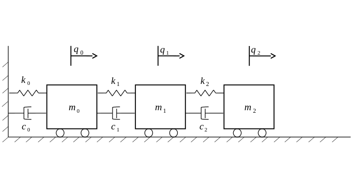
This notebook will introduce the class VibeSystem(), which is available in the vibration_toolbox. As an example we will use the following 3 degree of freedom system:

System

If we look at the help for the VibeSystem class we have:

Parameters
----------
M : array
    Mass matrix.
C : array
    Damping matrix.
K : array
    Stiffness matrix.
name : str, optional
    Name of the system.

So we need to get the mass, stiffness and damping matrix to create a VibeSystem object (the name of the system is optional and can be used latter to help when we plot results).

For this system the kinetic energy is:

\begin{equation} T = \frac{1}{2}[m_0\dot{q_0}(t)^2 + m_1\dot{q_1}(t)^2 + m_2\dot{q_2}(t)^2] = \frac{1}{2}{\bf \dot{q}}^T(t)\ M \ {\bf \dot{q}}(t) \end{equation}

where \({\bf q(t)} = [q_0(t) \ q_1(t) \ q_2(t)]^T\) is the configuration vector. The mass matrix for this system is given by:

\begin{equation} M = \begin{bmatrix} m_0 & 0 & 0\\ 0 & m_1 & 0 \\ 0 & 0 & m_2 \end{bmatrix} \end{equation}

The potential energy is:

\begin{equation} V = \frac{1}{2}[k_0 q_0(t)^2 + k_1(q_1(t) - q_0(t))^2 + k_2 (q_2(t) - q_1(t))^2] \end{equation}

\begin{equation} = \frac{1}{2}[(k_0+k_1)q_0(t)^2 + (k_1+k_2)q_1(t)^2 + (k_2)q_2(t)^2 -2k_1 q_0(t)q_1(t) - 2k_2 q_2(t)] \\ \end{equation}

\begin{equation} = \frac{1}{2}{\bf {q}}^T(t)\ K \ {\bf {q}}(t) \end{equation}

And the stiffness matrix is:

\begin{equation} K = \begin{bmatrix} k_0 +k_1 & -k_1 & 0\\ -k_1 & k_1+k_2 & -k_2 \\ 0 & -k_2 & k_2 \end{bmatrix} \end{equation}

In this case we will consider proportional damping: \(C = \alpha M + \beta K\).

Let’s consider the following values for our system:

m0, m1, m2 = (1, 1, 1)
k0, k1, k2 = (1600, 1600, 1600)
alpha, beta = 1e-3, 1e-3

Now we use numpy to create our matrices:

M = np.array([[m0, 0, 0],
              [0, m1, 0],
              [0, 0, m2]])
K = np.array([[k0+k1, -k1,   0],
              [-k1, k1+k2, -k2],
              [0,     -k2,  k2]])
C = alpha*M + beta*K

sys = vtb.VibeSystem(M, C, K, name='3 dof system')

Now we have everything needed to create a vibration system object:

Now, if we type ``sys.`` and press tab we can see the system’s attributes and methods that are available.

As an example we can get the natural frequencies:

sys.wn

array([ 17.80167472,  49.87918415,  72.07750943])

Or the damped natural frequencies:

sys.wd

array([ 17.80096508,  49.86365725,  72.03066935])

We can also check the frequency response for specific input output pairs:

ax = sys.plot_freq_response(0, 0)

M, C and K can be changed and the system will be updated:

sys.C = 20*C
sys.wd

array([ 17.51552471,  43.22562039,  49.95149484])

ax = sys.plot_freq_response(0, 0)

sys.C = C
axs = sys.plot_freq_response_grid([0, 1], [0, 1])

For the plot functions, the axes that will be used can be provided. This can help us when we want to show two different results on the same plot. This is ilustrated below by plotting the frequency response first using only the first two modes:

ax = sys.plot_freq_response(0, 0, modes=[0, 1],
                            color='r', linestyle='--',
                            label='Modes 0 and 1')

Notice that the axes with magnitude and phase were returned and assigned to the ‘ax’ name.

Now we pass ‘ax’ to plot the frequency response with all the modes (default when modes are not provided).

ax = sys.plot_freq_response(0, 0, ax0=ax[0], ax1=ax[1],
                            color='b', label='All modes')

We can check the results below:

ax = sys.plot_freq_response(0, 0, modes=[0, 1],
                            color='r', linestyle='--',
                            label='Modes 0 and 1')
ax = sys.plot_freq_response(0, 0, ax0=ax[0], ax1=ax[1],
                            color='b', label='All modes')
ax[1].legend();

The time response for the system can also be plotted. For that we need to define a time array and the force that will be applied during that time. The force should be given as an array where each row corresponds to a period of time and each column to where the force is being applied.

t = np.linspace(0, 25, 1000)
# force array with len(t) rows and len(inputs) columns
F1 = np.zeros((len(t), 3))
# in this case we apply the force only to the mass m1
F1[:, 1] = 1000*np.sin(40*t)

axs = sys.plot_time_response(F1, t)

We can use the plot_fft function available in the toolbox to see the FFT from the time response.

t, yout, xout = sys.time_response(F1, t)
ax = vtb.plot_fft(t, time_response=yout[:, 0])